Coordinate Mapping and Matrix Structure
Laser calibration patterns systematically vary two independent operational variables across an orthogonal grid. The horizontal axis typically increments travel speed in millimeters per second, while the vertical axis scales optical power duty cycle from minimal threshold to maximum rated current. Evaluating this matrix begins by verifying the intended baseline coordinate: the bottom-left corner generally marks the lowest energy density configuration, and the diagonal toward the top-right corresponds to the steepest energy concentration per unit surface area.
Failing to confirm the matrix coordinate orientation leads to inverted conclusions about material sensitivity. Operators must first verify whether speed increases left-to-right or right-to-left before evaluating line pitch and interval spacing. When evaluating a test coupon, always measure the outer perimeter with calipers to ensure the test program maintained true 1:1 dimensional proportionality without axis scaling errors.
Isolating Contrast From Thermal Bleed
Optical contrast represents one of the most misleading attributes when viewed without magnification. On dark anodized aluminum, a brilliant white engraving patch may indicate either cleanly ablated pigment or brittle re-melted aluminum oxide that easily flakes off after light ultrasonic cleaning. Reading a grid requires wiping the surface with isopropyl alcohol before grading cell clarity, ensuring that volatile organic soot does not pass for durable contrast.
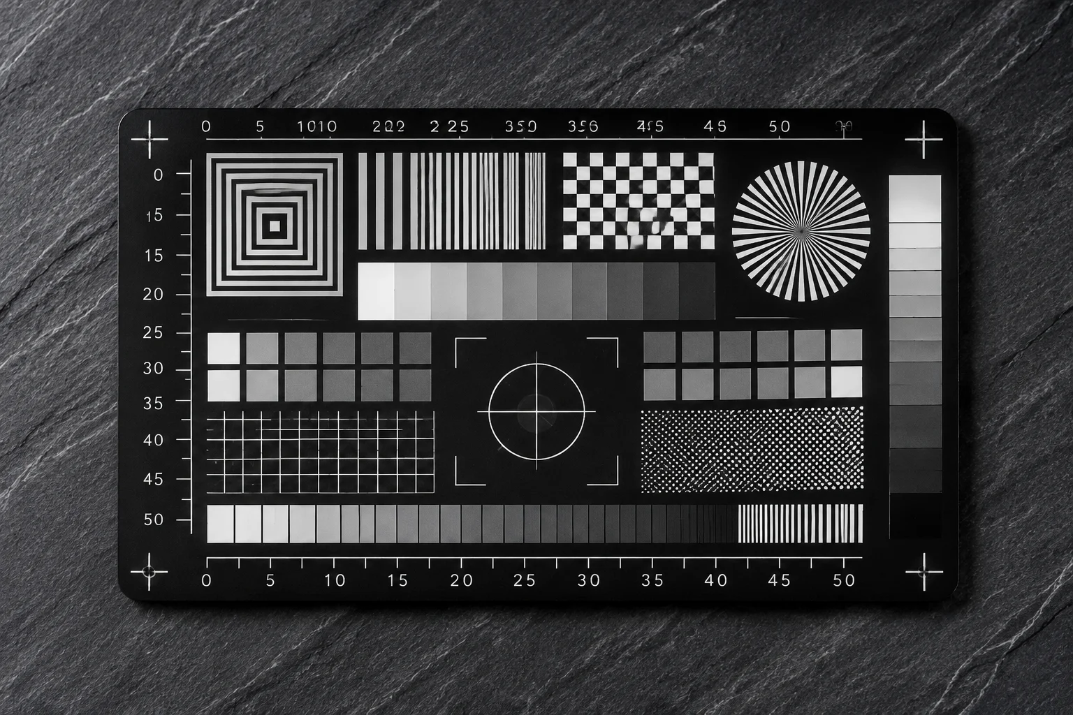
Thermal bleed manifests as a halo expanding beyond the programmed rectangular border into neighboring cells. When heat accumulates within the material core faster than surrounding conduction can dissipate it, adjacent tracks lose edge sharpness. The optimal parameter zone is located immediately after the threshold of uniform marking, well before adjacent squares show signs of heat bloom or edge roll-off.
Identifying Mechanical and Optical Artifacts
A test grid reveals not only chemical and thermal responses of the target medium, but also mechanical resonance from machine gantries and galvo mirror settling delays. High-speed cells often exhibit faded leading edges where the beam traversed the perimeter before reaching programmed pulse frequency, alongside darker trailing edges caused by mechanical dwell times during reversal maneuvers.
Critical Flaws Visible Under Direct Inspection
Inspecting individual test cells with oblique directional lighting highlights micro-topographical flaws invisible under diffuse illumination. Pay close attention to these three primary failure modes:
- Scanline banding caused by improper line intervals where the spot diameter leaves untreated ridges or creates excessive double-pulse overlap.
- Edge scalloping and corner rounding produced by aggressive acceleration parameters exceeding the mechanical damping of the axis motors.
- Surface carbonization and thermal craze cracking where excessive power density degrades polymers or causes micro-fracturing in mineral coats.
Translating Grid Coordinates Into Production Files
Selecting an operational recipe from a finished grid is never a matter of picking the single cell with the deepest mark. If that cell borders an area of severe burning or dimensional distortion, standard process variations such as substrate thickness tolerance or laser tube decay will push your production run directly into failure. The target parameter set must reside centrally within a cluster of at least three by three stable, acceptable cells.
Once a resilient cluster is pinpointed, log both nominal values and the ambient operating conditions into your laboratory ledger. Note the lens focal length, assist air pressure, workpiece thickness, and surface preparation. A grid reading remains valid only when the optical transmission train and workpiece environmental conditions match those present during the initial calibration trial.